Useful Solara Components (App Elements)
Applications are built in Solara using components. These are
modular, reusable, and maintainable user interface elements. Components
can be designed independently and combined to form more complex,
interactive applications. There are two main types: widget and
function. Widgets correspond to ipywidgets and function
components are responsible for combining logic, state, and more. When
seeing the term component, this generally refers to function.
Please see the Components documentation and API reference for more information.
Creating components typically includes defining a Python function and
decorating this function using @solara.component.
A variety of examples are shown below.
The Main Component
The main component of a Solara app holds the interface and can include
other components inside. This is commonly named Page(). In order to
create the main Page() component, it must be defined at the end of
the script and include a @solara.component decorator. If other
components are created inside the app’s code, Page() must be the
final component defined.
@solara.component
def Page():
    ...
If launching the Solara app as a .py file, Solara will render all
elements inside the Page() component. However, if using a .ipynb
file, display(Page()) will need to be included as the final line of
code.
# the following line is only necessary inside Jupyter notebook to render Page components
display(Page())
Hooks
Solara offers reusable hooks similar to those in the ReactJS ecosystem. For available hooks, please visit Solara’s API and Rules of Hooks
Interactive Widgets
Solara offers a wide variey of widgets by utilizing the entire
ipywidgets ecosystem. In addition to the elements shown here, users
can create custom widgets from Solara components (see details
here) and transition a pre-existing
application using pure ipywidgets to using
Reacton to wrap a
React-like layer around widgets (see details
here).
Button
The following code outlines the arguments that can be passed through
solara.Button(). In addition, an overview of icons can be found
here.
@solara.component
def Button(
    label: str = None,                      # text to display on button
    on_click: Callable[[], None] = None,    # callback function when button is clicked
    icon_name: str = None,                  # name of icon to display on button
    children: list = [],                    # list of child elements to display on button
    disabled=False,                         # whether button is disabled
    text=False,                             # display button as text only
    outlined=False,                         # display button outline only with text
    color: Optional[str] = None,
    classes: List[str] = [],                # additional CSS classes to apply
    style: Union[str, Dict[str, str], None] = None,     # CSS styles to apply
    value=None,                             # value when used as child of toggle button component
    **kwargs,
):
Create a button by using solara.Button() inside the Page()
component.
import solara

@solara.component
def Page():
    with solara.Row():  # optional row layout to display the following buttons
        solara.Button(label="Default")
        solara.Button(label="Default+color", color="primary")
        solara.Button(label="Text", text=True)
        solara.Button(label="Outlined", outlined=True)
        solara.Button(label="Outlined+color", outlined=True, color="primary")

# the following line is only necessary inside Jupyter notebook to render Page components
display(Page())
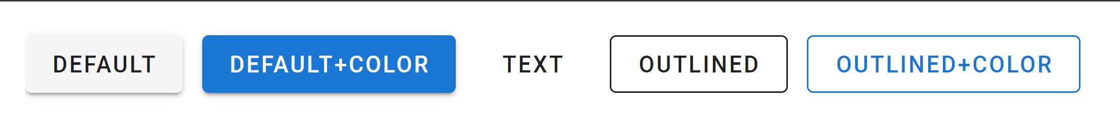
A screenshot of various button types
Checkbox
The following code outlines the arguments that can be passed through
solara.Checkbox().
@reacton.value_component(bool)
def Checkbox(
    *,
    label=None,                                         # label to display next to checkbox
    value: Union[bool, solara.Reactive[bool]] = True,   # initial boolean value of checkbox
    on_value: Callable[[bool], None] = None,            # callback when checkbox is toggled
    disabled=False,                                     # whether to disable checkbox use
    style: str = None,                                  # string of CSS styles to apply to checkbox
):

    ...
First, initialize a reactive variable using solara.reactive()
outside of any Solara components.
cb = solara.reactive(True)
Then, use solara.Checkbox() inside the Page() component with the
value set to the reactive variable defined above.
import solara

# initialize reactive variable
cb = solara.reactive(True)

@solara.component
def Page():
    # render a checkbox
    solara.Checkbox(label="Check me!", value=cb)

    # use the checkbox state to display the appropriate text
    if cb.value:
        solara.Markdown("The box is checked")
    else:
        solara.Markdown("The box is not checked")

# the following line is only necessary inside Jupyter notebook to render Page components
display(Page())

A gif of a checkbox
Select
Solara offers a dropdown selection widget with the ability to select single or multiple items.
The following code outlines the arguments that can be passed through
solara.Select().
@solara.value_component(None)
def Select(
    label: str,                                         # label to display next to the selection widget
    values: List[T],                                    # list of all selectable values
    value: Union[None, T, solara.Reactive[T], solara.Reactive[Optional[T]]] = None,     # actively selected value
    on_value: Union[None, Callable[[T], None], Callable[[Optional[T]], None]] = None,   # callback upon value change
    dense: bool = False,                                # whether to use a denser style
    disabled: bool = False,                             # whether to allow user interaction
    classes: List[str] = [],                            # list of CSS classes to apply to the widget
    style: Union[str, Dict[str, str], None] = None,     # CSS style to apply to the widget
) -> reacton.core.ValueElement[v.Select, T]:

    ...
The following code outlines the arguments that can be passed through
solara.SelectMultiple().
@solara.value_component(None)
def SelectMultiple(
    label: str,                                         # label to display next to the selection widget
    values: List[T],                                    # list of actively selected values
    all_values: List[T],                                # list of all selectable values
    on_value: Callable[[List[T]], None] = None,         # callback upon value change
    dense: bool = False,                                # whether to use a denser style
    disabled: bool = False,                             # whether to allow user interaction
    classes: List[str] = [],                            # list of CSS classes to apply to the widget
    style: Union[str, Dict[str, str], None] = None,     # CSS style to apply to the widget
) -> reacton.core.ValueElement[v.Select, List[T]]:

    ...
The following code demonstrates both modes of selection widgets.
import solara

fruits = ["Kiwi", "Banana", "Apple"]
fruit = solara.reactive(None)       # sets initial selection to None

veggies_all = ["Broccoli", "Celery", "Carrot"]
veggies = solara.reactive(None)     # sets initial selection to None

@solara.component
def Page():
    solara.Select(label="Single Fruit", value=fruit, values=fruits)
    solara.Markdown(f"**Selected**: {fruit.value}")             # reactive text displaying selection

    solara.SelectMultiple("Multiple Vegetables", veggies, veggies_all)
    solara.Markdown(f"**Selected**: {veggies.value}")           # reactive text displaying selection(s)

# the following line is only necessary inside Jupyter notebook to render Page components
display(Page())
A gif showing both modes of selection widgets
Slider
Solara offers slider widgets for many different types of data. These include sliders for both numerical and non-numerical values, such as dates and strings.
Slider for Single Selection of Integers or Float Values
The following code outlines the arguments that can be passed through
solara.SliderInt().
@solara.value_component(int)
def SliderInt(
    label: str,
    value: Union[int, solara.Reactive[int]] = 0,
    min: int = 0,
    max: int = 10,
    step: int = 1,
    on_value: Optional[Callable[[int], None]] = None,
    thumb_label: Union[bool, Literal["always"]] = True,
    tick_labels: Union[List[str], Literal["end_points"], bool] = False,
    disabled: bool = False,
):

    ...
The following code outlines the arguments that can be passed through
solara.SliderFloat().
@solara.value_component(float)
def SliderFloat(
    label: str,
    value: Union[float, solara.Reactive[float]] = 0,
    min: float = 0,
    max: float = 10.0,
    step: float = 0.1,
    on_value: Callable[[float], None] = None,
    thumb_label: Union[bool, Literal["always"]] = True,
    tick_labels: Union[List[str], Literal["end_points"], bool] = False,
    disabled: bool = False,
):

    ...
A reactive variable must be initialized using solara.reactive() with
a default value defined and placed outside the Page() component.
int_value = solara.reactive(42)         # for integer
float_value = solara.reactive(42.4)     # for float value
To use a slider for integers, solara.SliderInt() is placed inside
Page(). To use a slider for float values, solara.SliderFloat()
is used instead.
solara.SliderInt("Integer", value=int_value, min=-10, max=120)          # for integer
solara.SliderFloat("Float Value", value=float_value, min=-10, max=120)  # for float value
The following code renders a separate slider for integer and float value selection, markdown text displaying the value selected beneath each respective slider, and a respective reset button to restore the value to default.
import solara

# initialize reactive variable and set default value
int_value = solara.reactive(42)
float_value = solara.reactive(42.4)

@solara.component
def Page():
    # Integers
    solara.SliderInt("Integer", value=int_value, min=-10, max=120)
    solara.Markdown(f"**Int value**: {int_value.value}")
    with solara.Row():
        solara.Button("Reset", on_click=lambda: int_value.set(42))

    # Float Values
    solara.SliderFloat("Float Value", value=float_value, min=-10, max=120)
    solara.Markdown(f"**Float value**: {float_value.value}")
    with solara.Row():
        solara.Button("Reset", on_click=lambda: float_value.set(42.5))

# the following line is only necessary inside Jupyter notebook to render Page components
display(Page())
A gif showing slider widgets for individual numbers
Slider for Range of Integers or Float Values
The following code outlines the arguments that can be passed through
solara.SliderRangeInt().
@solara.value_component(None)
def SliderRangeInt(
    label: str,
    value: Union[Tuple[int, int], solara.Reactive[Tuple[int, int]]] = (1, 3),
    min: int = 0,
    max: int = 10,
    step: int = 1,
    on_value: Callable[[Tuple[int, int]], None] = None,
    thumb_label: Union[bool, Literal["always"]] = True,
    tick_labels: Union[List[str], Literal["end_points"], bool] = False,
    disabled: bool = False,
) -> reacton.core.ValueElement[ipyvuetify.RangeSlider, Tuple[int, int]]:

    ...
The following code outlines the arguments that can be passed through
solara.SliderRangeFloat().
@solara.value_component(None)
def SliderRangeFloat(
    label: str,
    value: Union[Tuple[float, float], solara.Reactive[Tuple[float, float]]] = (1.0, 3.0),
    min: float = 0.0,
    max: float = 10.0,
    step: float = 0.1,
    on_value: Callable[[Tuple[float, float]], None] = None,
    thumb_label: Union[bool, Literal["always"]] = True,
    tick_labels: Union[List[str], Literal["end_points"], bool] = False,
    disabled: bool = False,
) -> reacton.core.ValueElement[ipyvuetify.RangeSlider, Tuple[float, float]]:

    ...
A reactive variable must be initialized using solara.reactive() with
default range values defined and placed outside the Page()
component.
int_range = solara.reactive((0, 42))            # for integer range
float_range = solara.reactive((0.1, 42.4))      # for float range
To use a slider to define a range of integers,
solara.SliderRangeInt() is placed inside Page(). To use a slider
to define a range of float values, solara.SliderRangeFloat() is used
instead.
solara.SliderRangeInt("Some integer range", value=int_range, min=-10, max=120)      # for integer range
solara.SliderRangeFloat("Some float range", value=float_range, min=-10, max=120)    # for float range
The following code renders a separate slider for range selection of integers and float values, markdown text displaying the chosen range beneath each respective slider, and reset buttons to restore the slider to the default ranges.
import solara

# initialize reactive variable and set default value
int_range = solara.reactive((0, 42))
float_range = solara.reactive((0.1, 42.4))

@solara.component
def Page():
    # Integers
    solara.SliderRangeInt("Some integer range", value=int_range, min=-10, max=120)
    solara.Markdown(f"**Int range value**: {int_range.value}")
    with solara.Row():
        solara.Button("Reset", on_click=lambda: int_range.set((0, 42)))

    # Float Values
    solara.SliderRangeFloat("Some float range", value=float_range, min=-10, max=120)
    solara.Markdown(f"**Float range value**: {float_range.value}")
    with solara.Row():
        solara.Button("Reset", on_click=lambda: float_range.set((0.1, 42.4)))

# the following line is only necessary inside Jupyter notebook to render Page components
display(Page())
A gif showing slider widgets for numerical ranges
Slider for Categorical Values
The following code outlines the arguments that can be passed through
solara.SliderValue().
@solara.value_component(None)
def SliderValue(
    label: str,
    value: Union[T, solara.Reactive[T]],
    values: List[T],
    on_value: Callable[[T], None] = None,
    disabled: bool = False,
) -> reacton.core.ValueElement[ipyvuetify.Slider, T]:

    ...
A reactive variable must first be initialized using
solara.reactive("default value") with a default value specified.
This line is placed outside of the Page() component.
fruits = ["Kiwi", "Banana", "Apple"]
fruit = solara.reactive("Banana")       # initialize reactive variable and set default value
Next, solara.SliderValue() is placed inside Page() to render the
slider in your app.
solara.SliderValue(label="Fruit", value=fruit, values=fruits)
The following code will render a slider widget and markdown text displaying the selected value beneath.
import solara

fruits = ["Kiwi", "Banana", "Apple"]
fruit = solara.reactive("Banana")       # initialize reactive variable and set default value

@solara.component
def Page():
    solara.SliderValue(label="Fruit", value=fruit, values=fruits)
    solara.Markdown(f"**Selected**: {fruit.value}")     # display selected value

# the following line is only necessary inside Jupyter notebook to render Page components
display(Page())
A gif showing a value slider widget
Slider for Dates
The following code outlines the arguments that can be passed through
solara.SliderDate().
@solara.value_component(date)
def SliderDate(
    label: str,                                 # label to display next to slider
    value: Union[date, solara.Reactive[date]] = date(2010, 7, 28),     # selected value
    min: date = date(1981, 1, 1),               # minimum value
    max: date = date(2050, 12, 30),             # maximum value
    on_value: Callable[[date], None] = None,    # callback upon value change
    disabled: bool = False,                     # whether slider is disabled
):

    ...
In order to utilize the slider widget for date selection, the
datetime library will need to be imported. A default date (e.g.,
date_default) can be set, and a reactive date variable (e.g.,
date_value) needs to be initialized using solara.reactive().
import datetime

date_default = datetime.date(2023, 10, 13)  # set default date
date_value = solara.reactive(date_default)  # initialize reactive variable
Next, solara.SliderDate() can be placed inside the Page()
component to render in your app.
solara.SliderDate("Some date", value=date_value)
The following code will render a date slider, markdown text displaying the date selected beneath the slider, and a reset button to restore the value to default.
import solara
import datetime

date_default = datetime.date(2023, 10, 13)  # set default date
date_value = solara.reactive(date_default)  # initialize reactive variable

@solara.component
def Page():
    # date slider widget
    solara.SliderDate("Some date", value=date_value)

    # display selected date
    solara.Markdown(f"**Date value**: {date_value.value.strftime('%Y-%b-%d')}")

    # reset button to restore slider to the default date
    with solara.Row():
        solara.Button("Reset", on_click=lambda: date_value.set(datetime.date(2010, 7, 28)))

# the following line is only necessary inside Jupyter notebook to render Page components
display(Page())
Note: The date displayed to the right of the slider and the value stored are off by one day. See reported issue #409.

A gif showing a date slider widget
Toggle Switch
Solara offers a switch component that can be toggled on and off. The
following code outlines the arguments that can be passed through
solara.Switch().
@solara.value_component(bool)
def Switch(
    *,
    label: str = None,
    value: Union[bool, solara.Reactive[bool]] = True,
    on_value: Callable[[bool], None] = None,
    disabled: bool = False,
    children: list = [],
    classes: List[str] = [],
    style: Optional[Union[str, Dict[str, str]]] = None,
):

    ...
A reactive variable must first be defined before the Page()
component using solara.reactive(). A default boolean state (i.e.,
True or False) must also be defined.
The following code shows an example of two reactive variables that hold a value for each switch.
show_message = solara.reactive(True)
disable = solara.reactive(False)
Inside the Page() component, solara.Switch() can be used with a
descriptive label and reactive value defined above. In addition,
switches can be linked such that one gets disabled by the state of
another. This is demonstrated below, where disabled=disabled.value
is passed through the first switch. Depending on the value of the second
switch, the first switch may or may not be disabled from use.
solara.Switch(label="Hide Message", value=show_message, disabled=disable.value)
solara.Switch(label="Disable Message Switch", value=disable)
The following code renders the above example, where user interaction of one switch is dependent on the state of the other switch.
import solara

# initialize reactive variables and set default boolean states
show_message = solara.reactive(True)
disable = solara.reactive(False)

@solara.component
def Page():
    with solara.Column():   # optional column layout
        with solara.Row():  # optional row layout
            solara.Switch(label="Hide Message", value=show_message, disabled=disable.value)
            solara.Switch(label="Disable Message Switch", value=disable)

        if show_message.value:
            solara.Markdown("## Use Switch to show/hide message")

# the following line is only necessary inside Jupyter notebook to render Page components
display(Page())

A gif showing switch widgets in action
Toggle Buttons
Solara offers toggle buttons for single and multiple selection of
values. Values can be passed as a list or through custom buttons
(children).
Toggle Buttons: Multiple Selection
The following code outlines the arguments that can be passed through
solara.ToggleButtonsMultiple().
@solara.value_component(None)
def ToggleButtonsMultiple(
    value: Union[List[T], solara.Reactive[List[T]]] = [],
    values: List[T] = [],
    children: List[reacton.core.Element] = [],
    on_value: Union[Callable[[List[T]], None], None] = None,
    dense: bool = False,
    mandatory: bool = False,
    classes: List[str] = [],
    style: Union[str, Dict[str, str], None] = None,
) -> reacton.core.ValueElement[v.BtnToggle, List[T]]:

    ...
First define reactive variables prior to the Page() component and
provide default value(s).
fruits = ["Kiwi", "Banana", "Apple"]    # list of values
fruit = solara.reactive([fruits[0]])    # reactive variable initialization
Next, use solara.ToggleButtonsMultiple() inside the Page()
component.
solara.ToggleButtonsMultiple(value=fruit, values=fruits)
The following example code will render a toggle button widget that enables multiple selection of options provided by the list of values.
import solara

fruits = ["Kiwi", "Banana", "Apple"]    # list of values
fruit = solara.reactive([fruits[0]])    # reactive variable initialization

@solara.component
def Page():
    with solara.Card("My favorite fruits"):   # optional card layout element
        solara.ToggleButtonsMultiple(value=fruit, values=fruits)
        solara.Markdown(f"**Selected**: {fruit.value}")

# the following line is only necessary inside Jupyter notebook to render Page components
display(Page())

A gif showing a multi-selection toggle widget
Input Fields
Solara offers an input field widget for visible and hidden (i.e., password) text, as well as numberical values.
Text Input
The following code outlines the arguments that can be passed through
solara.InputText().
@solara.component
def InputText(
    label: str,
    value: Union[str, solara.Reactive[str]] = "",
    on_value: Callable[[str], None] = None,
    disabled: bool = False,
    password: bool = False,
    continuous_update: bool = False,
    update_events: List[str] = ["blur", "keyup.enter"],
    error: Union[bool, str] = False,
    message: Optional[str] = None,
    classes: List[str] = [],
    style: Optional[Union[str, Dict[str, str]]] = None,
):

    ...
First, define reactive variables using solara.reactive() after
importing any dependencies.
text = solara.reactive("hello world")
pw = solara.reactive("goodbye world")
contup = solara.reactive(True)
Then, use solara.InputText() inside the Page() component to
render input fields. By default, password=False so text will be
visible while typed. To hide characters, use password=True.
solara.InputText("Enter some text", value=text, continuous_update=contup.value)
solara.InputText("Enter a passsword", value=pw, continuous_update=contup.value, password=True)
The following example demonstrates use of both standard and password input fields.
import solara

# initialize reactive variable and set default value(s)
text = solara.reactive("hello world")
pw = solara.reactive("goodbye world")
contup = solara.reactive(True)

@solara.component
def Page():
    solara.Checkbox(label="Continuous update", value=contup)

    # Text field where specific text is displayed
    solara.InputText("Enter some text", value=text, continuous_update=contup.value)

    # optional addition of a clear and reset button
    with solara.Row():
        solara.Button("Clear", on_click=lambda: text.set(""))
        solara.Button("Reset", on_click=lambda: text.set("hello world"))
    solara.Markdown(f"**You entered**: {text.value}")

    # Password field where specific text characters are not displayed
    solara.InputText("Enter a passsword", value=pw, continuous_update=contup.value, password=True)

    # optional addition of a clear and reset button
    with solara.Row():
        solara.Button("Clear", on_click=lambda: pw.set(""))
        solara.Button("Reset", on_click=lambda: pw.set("goodbye world"))
    solara.Markdown(f"**You entered**: {pw.value}")

# the following line is only necessary inside Jupyter notebook to render Page components
display(Page())

A gif of the text input widgets
Numerical Input
For numerical input fields, use solara.InputFloat() or
solara.InputInt() instead.
File Handling
File Drop
Solara enables file dropping, a convenient way to upload local files. See details here.
The following code outlines the arguments that can be passed through
solara.FileDrop(). If lazy=True, file content will neither be
loaded into memory nor transferred by default. Data will be transferred
as needed when a file object is passed through with the on_file
callback. If lazy=False, file content will be loaded into memory and
passed to the on_file callback through the .data attribute. The
on_file argument is called with a FileInfo object which contains
the file .name, .length, and .file_obj object, as well as
.data if lazy=False.
@solara.component
def FileDrop(
    label="Drop file here",
    on_total_progress: Optional[Callable[[float], None]] = None,    # calls progress percentage of file upload
    on_file: Optional[Callable[[FileInfo], None]] = None,           # called with `FileInfo` object
    lazy: bool = True,
):

    ...
The following code will generate a file drop region that reads the first 100 bytes of file data.
Note: Although the file drop region renders inside Jupyter notebook,
it is not fully functional. The File Dropper works best when launch
Solara apps directly from .py files.
import solara
from solara.components.file_drop import FileInfo
import textwrap


@solara.component
def Page():
    content, set_content = solara.use_state(b"")
    filename, set_filename = solara.use_state("")
    size, set_size = solara.use_state(0)

    def on_file(file: FileInfo):
        set_filename(file["name"])
        set_size(file["size"])
        f = file["file_obj"]
        set_content(f.read(100))

    with solara.Div() as main:
        solara.FileDrop(
            label="Drag and drop a file here to read the first 100 bytes",
            on_file=on_file,
            lazy=True,  # We will only read the first 100 bytes
        )
        if content:
            solara.Info(f"File {filename} has total length: {size}\n, first 100 bytes:")
            solara.Preformatted("\n".join(textwrap.wrap(repr(content))))

    return main

# the following line is only necessary inside Jupyter notebook to render Page components
display(Page())

A gif showing the file dropper in action
File Browser
The following code outlines the arguments that can be passed through
solara.FileBrowser(). See details
here.
Enabling selection using can_select=True allows a file or folder to
be highlighted with the first click and opened with a double click.
Disabling selection using can_select=False allows a file or folder
to be opened with a single click. These modes also determine the
behavior of on_directory_change, on_path_select, and
on_file_open arguments.
@solara.component
def FileBrowser(
    directory: Union[None, str, Path, solara.Reactive[Path]] = None,    # starting directory
    on_directory_change: Callable[[Path], None] = None,                 # triggered with 1 or 2 clicks on a directory (depends on `can_select`)
    on_path_select: Callable[[Optional[Path]], None] = None,            # never triggered or triggered by clicking on a file or directory (depends on `can_select`)
    on_file_open: Callable[[Path], None] = None,                        # triggered with 1 or 2 clicks on a file or directory (depends on `can_select`)
    filter: Callable[[Path], bool] = lambda x: True,                    # a function that takes a `Path`` and returns `True` if the file/directory should be shown
    directory_first: bool = False,                                      # if `True`, directories are shown before files
    can_select=False,                                                   # sets single or double click mode of selecting a file or directory
):

    ...
State management with solara.use_state() needs to be incorporated
for reactive updates to the file, path, and directory
information as the user clicks through the file browser. To do so,
include the following lines in the dependencies:
from pathlib import Path
from typing import Optional, cast
Then, initialize reactive variables with the following code, placed
inside the Page() component:
file, set_file = solara.use_state(cast(Optional[Path], None))
path, set_path = solara.use_state(cast(Optional[Path], None))
directory, set_directory = solara.use_state(Path("~").expanduser())

solara.FileBrowser(directory, on_directory_change=set_directory, on_path_select=set_path, on_file_open=set_file)
The following example shows sample code needed to render the file browser in Solara:
import solara
from pathlib import Path
from typing import Optional, cast

@solara.component
def Page():
    # reactive variables using state management
    file, set_file = solara.use_state(cast(Optional[Path], None))
    path, set_path = solara.use_state(cast(Optional[Path], None))
    directory, set_directory = solara.use_state(Path("~").expanduser())

    # Vertical Box (VBox) wrapper; not critical for functionality
    with solara.VBox() as main:
        solara.FileBrowser(directory, on_directory_change=set_directory, on_path_select=set_path, on_file_open=set_file)
    return main

# the following line is only necessary inside Jupyter notebook to render Page components
display(Page())

A gif showing the file browser rendered in Solara
File Downloader
Solara enables a widget to download data, which can be a string, bytes,
a file-like object, or even a function that returns the aforementioned.
With solara.FileDownload(), Solara renders a standard download
button which can be customized by providing children. Children can
be any solara component, including another button, markdown text, or an
image. It may be helpful to note that data is kept in the session memory
when downloading. See details
here.
Note: When using Solara in Jupyter notebooks through a VS Code instance on Notebooks Hub, VS Code will prompt the user to save the file on the server.
The following code outlines the arguments that can be passed through
solara.FileDownload(). In addition, an overview of icons can be
found here.
@solara.component
def FileDownload(
    data: Union[str, bytes, BinaryIO, Callable[[], Union[str, bytes, BinaryIO]]],   # data to download
    filename: Optional[str] = None,                             # default filename of downloaded data
    label: Optional[str] = None,                                # label of button
    icon_name: Optional[str] = "mdi-cloud-download-outline",    # name of icon to display on button
    close_file: bool = True,                                    # if file object is provided, close file after downloading
    mime_type: str = "application/octet-stream",                # mime type of file
    string_encoding: str = "utf-8",                             # encoding to use when converting a string to bytes
    children=[],                                                # for customizing the clickable object
):

    ...
To display a download button, solara.FileDownload() can be placed
inside Page(). The label argument enables custom text to be
displayed on the button.
solara.FileDownload(data, filename="solara-download.txt", label="Download file")
The following code shows four different clickable objects that trigger file download.
import solara

data = "This is the content of the file"

@solara.component
def Page():
    # standard download button
    solara.FileDownload(data, filename="solara-download.txt", label="Download file")

    # clickable text to trigger download
    with solara.FileDownload(data, "solara-download-2.txt"):
        solara.Markdown("clickable text")

    # clickable image to trigger download
    with solara.FileDownload(data, "solara-download-3.txt"):
        solara.Image("https://solara.dev/static/public/beach.jpeg", width="200px")

    # custom download button
    with solara.FileDownload(data, "solara-download-4.txt"):
        solara.Button("Custom download button", icon_name="mdi-cloud-download-outline", color="primary")

# the following line is only necessary inside Jupyter notebook to render Page components
display(Page())

A screenshot showing four download “button” options
The following code shows a file-like object being used as data for
download. In addition, the example sets mime_type to
application/vnd.ms-excel. If the Solara application is rendered
outside of a Jupyter notebook, this would allows the user OS to directly
open the file in Excel.
import solara
import pandas as pd

df = pd.DataFrame({"id": [1, 2, 3], "name": ["John", "Mary", "Bob"]})

@solara.component
def Page():
    file_object = df.to_csv(index=False)
    solara.FileDownload(file_object, "users.csv", mime_type="application/vnd.ms-excel")

# the following line is only necessary inside Jupyter notebook to render Page components
display(Page())

A screenshot showing the file download button
DataFrames
Solara apps can display Pandas dataframes inside a table using
solara.DataFrame(). The following code outlines the arguments that
can be passed through solara.DataFrame().
@solara.component
def DataFrame(
    df,     # pandas dataframe
    items_per_page=20,  # optional specification
    column_actions: List[ColumnAction] = [],    # triggered when clicking on triple dots that appear upon hovering
    cell_actions: List[CellAction] = [],        # triggered when clicking on triple dots that appear upon hovering
    scrollable=False,
    on_column_header_hover: Optional[Callable[[Optional[str]], None]] = None,   # optional callback upon hovering over triple dots
    column_header_info: Optional[solara.Element] = None,                        # element displayed upon hovering over triple dots
):

    ...
Basic Pandas DataFrame
To display a Pandas dataframe, use solara.DataFrame() and pass in a
dataframe as the first argument, optionally followed by the number of
items to be displayed per table page.
The single line of code should appear:
solara.DataFrame(df, items_per_page=5)
The line of code shown above can then be placed inside a component, such
as Page(), similar to that shown below:
import solara
import plotly
# import pandas as pd   # included for completeness

df = plotly.data.iris() # pandas dataframe (sourced from plotly)

@solara.component
def Page():
    solara.DataFrame(df, items_per_page=5)  # line of code to display pandas dataframe

# the following line is only necessary inside Jupyter notebook to render Page components
display(Page())
A gif showing the output of a simple dataframe
DataFrames with Column Header Tools
In addition, custom components can be added for increased interaction with the dataframe once the dataframe is rendered.
The column_header_info argument displays a custom component (i.e.,
box) when the user hovers over the column header with the mouse pointer.
For example, the following code will display a text box showing counts for each unique value inside the column that is being hovered over:
# set initial empty state to provide an empty container
column_hover, set_column_hover = solara.use_state(None)

with solara.Column(margin=4) as column_header_info:             # sets a solara.Column container as the column_header_info
        if column_hover:
            solara.Text("Value counts for " + column_hover)     # display text and name of column hovered
            display(df[column_hover].value_counts())            # display counts of unique values of column hovered
solara.DataFrame() can be updated to include
column_header_info and on_column_header_hover.solara.Column was used to define
column_header_info, so
column_header_info = column_header_info. This enables the triple
dot icon to appear upon hovering over.on_column_header_hover is an optional callback
used when the user hovers the triple dots in each column. This
argument is set to set_column_hover and enables
column_header_info to be displayed. When set to None, an empty
container appears instead.solara.DataFrame(df, column_header_info=column_header_info, on_column_header_hover=set_column_hover)
These lines of code can now be incorporated into a component, such as
Page(), similar to that shown below:
import solara
import plotly
# import pandas as pd   # included for completeness

df = plotly.data.iris()

@solara.component
def Page():
    column_hover, set_column_hover = solara.use_state(None)

    with solara.Column(margin=4) as column_header_info:
        if column_hover:
            solara.Text("Value counts for " + column_hover)
            display(df[column_hover].value_counts())

    solara.DataFrame(df, column_header_info=column_header_info, on_column_header_hover=set_column_hover)

# the following line is only necessary inside Jupyter notebook to render Page components
display(Page())
A gif showing output of dataframe with custom column headers
Cross Filtering
Cross filtering collects a set of filters and combines them into one
filter to wrap a pandas dataframe. See details on the
use_cross_filter hook
here.
To use cross filtering, add solara.provide_cross_filter() inside a
component, such as Page(). Then, incorporate any of the related
widgets shown below. These widgets are best used in combination with
each other.
Display Filtered DataFrame
The following code outlines the arguments that can be passed through
solara.CrossFilterDataFrame().
@solara.component
def CrossFilterDataFrame(
    df,                                         # dataframe to which filter is applied
    items_per_page=20,                          # optional specification
    column_actions: List[ColumnAction] = [],    # triggered when clicking on triple dots that appear upon hovering
    cell_actions: List[CellAction] = [],        # triggered when clicking on triple dots that appear upon hovering
    scrollable=False
):

    ...
The following line of code is the simplest that can be incorporated
inside a component (e.g., Page()) to display a dataframe that
updates with each cross filter applied:
solara.CrossFilterDataFrame(df)
The following code demonstrates the addition of
solara.CrossFilterDataFrame() inside Page(). Without the
addition of other cross filtering widgets, the output is similar to that
which simply displays a pandas dataframe.
import solara
import plotly

df = plotly.data.gapminder()

@solara.component
def Page():
    solara.provide_cross_filter()       # enables crossfilter use
    solara.CrossFilterDataFrame(df)     # display filtered dataframe

# the following line is only necessary inside Jupyter notebook to render Page components
display(Page())
A gif of the cross filter dataframe
Display the Number of Filtered Rows over the Total Number of Rows
The following code outlines the arguments that can be passed through
solara.CrossFilterReport(). This widget displays the total number of
dataframe rows that remain after applying cross filters. The reported
count changes by updating cross filters using the other cross filtering
widgets (i.e., CrossFilterSelect() and CrossFilterSlider()).
@solara.component
def CrossFilterReport(
    df,                         # dataframe to which filter is applied
    classes: List[str] = []     # additional CSS classes to add to main widget; optional.
):

    ...
The following line of code can be incorporated inside a component (e.g.,
Page()) to report the number of rows filtered:
solara.CrossFilterReport(df, classes=["py-2"])
The following code demonstrates the addition of
solara.CrossFilterReport() inside Page(). Without the addition
of other cross filtering widgets, the output simply displays the total
number of rows in the dataframe passed through.
import solara
import plotly

df = plotly.data.gapminder()

@solara.component
def Page():
    solara.provide_cross_filter()                       # enables crossfilter use
    solara.CrossFilterReport(df, classes=["py-2"])      # indicator that reports number of rows selected using crossfilter over the total

# the following line is only necessary inside Jupyter notebook to render Page components
display(Page())

A screenshot of the cross filter reporter
Display Dropdown Selection Widget For Categorical Filtering
The following code outlines the arguments that can be passed through
solara.CrossFilterSelect().
@solara.component
def CrossFilterSelect(
    df,                         # dataframe to which filter is applied
    column: str,                # column to filter on
    max_unique: int = 100,      # maximum number of unique values to show in the dropdown widget
    multiple: bool = False,     # whether to allow multiple selection of values
    invert=False,               # whether to invert the selection
    configurable=True,          # whether to show the configuration button to the user
    classes: List[str] = [],    # additional CSS classes to add to the main widget
):

    ...
The following line of code can be incorporated inside a component (e.g.,
Page()) to display a dropdown selection widget for categorical
filtering:
solara.CrossFilterSelect(df, "country")
The following code demonstrates the addition of
solara.CrossFilterSelection() inside Page(). Without the
addition of other cross filtering widgets, the output simply displays
the dropdown widget.
import solara
import plotly

df = plotly.data.gapminder()

@solara.component
def Page():
    solara.provide_cross_filter()                       # enables crossfilter use
    solara.CrossFilterSelect(df, "country")             # filter using dropdown selection

# the following line is only necessary inside Jupyter notebook to render Page components
display(Page())

A gif of the cross filter dropdown selector
Display Slider Widget For Numerical Filtering
The following code outlines the arguments that can be passed through
solara.CrossFilterSlider(). The mode argument allows the
following relational options: == (equals to), >= (is greater
than or equal to), <= (is less than or equal to), > (is greater
than), and < (is less than).
@solara.component
def CrossFilterSlider(
    df,                     # dataframe to which filter is applied
    column: str,            # column to filter on
    invert=False,           # whether to invert the selection
    enable: bool = True,    # whether to enable (True) or disable (False) the filter
    mode: str = "==",       # the mode to use for filtering: ==, >=, <=, >, <.
    configurable=True,      # whether to show the configuration button to the user
):

    ...
The following line of code can be incorporated inside a component (e.g.,
Page()) to display a slider to filter using a numerical threshold:
solara.CrossFilterSlider(df, "pop", mode=">")
The following code demonstrates the addition of
solara.CrossFilterSlider() inside Page(). Without the addition
of other cross filtering widgets, the output simply displays the slider.
import solara
import plotly

df = plotly.data.gapminder()

@solara.component
def Page():
    solara.provide_cross_filter()                       # enables crossfilter use
    solara.CrossFilterSlider(df, "pop", mode=">")       # filter using slider

# the following line is only necessary inside Jupyter notebook to render Page components
display(Page())
A gif of the cross filter slider
Combining Cross Filtering Widgets
Now, all the cross filtering widgets described above can be combined in
any combination. The following code is an example that uses one of each
related widget and wraps them inside an optional vertical box container.
Although specific columns are identified in the code (i.e., country
and pop), the default argument includes configurable=True, which
enables the user to manually change the filtered columns once the
widgets are rendered.
import solara
import plotly

df = plotly.data.gapminder()

@solara.component
def Page():
    solara.provide_cross_filter()       # enables crossfilter use
    with solara.VBox() as main:         # Vertical Box (VBox) wrapper; not critical for functionality
        solara.CrossFilterReport(df, classes=["py-2"])      # indicator that reports number of rows selected using crossfilter over the total
        solara.CrossFilterSelect(df, "country")             # filter using dropdown selection
        solara.CrossFilterSlider(df, "pop", mode=">")       # filter using slider
        solara.CrossFilterDataFrame(df)                     # display filtered dataframe
    return main

# the following line is only necessary inside Jupyter notebook to render Page components
display(Page())
A gif of all cross filter widgets
Plots
Solara offers many ways to plot and visualize data. Supported libraries include Plotly, Matplotlib, Altair, and more.
Plotly and Plotly Express
Solara supports both plotly and plotly express. User events (e.g., data selection, hovers) and annotations are also supported.
The following code outlines the arguments that can be passed through
solara.FigurePlotly().
solara.FigurePlotly(
    fig,                                # figure object
    on_selection=set_selection_data,    # triggered when using selection tools to select data points
    on_click=set_click_data,            # triggered when clicking on data point
    on_hover=set_hover_data,            # triggered when hovering over data point
    on_unhover=set_unhover_data,        # triggered when unhovering from hovered data point
    on_deselect=set_deselect_data       # triggered when unselecting data points previously selected with selection tool
)
First, create a figure (not a figure widget) and pass it through the
FigurePlotly component using solara.FigurePlotly(). In the example
below, fig = px.scatter() creates a scatter plot object using
dataframe df, sepal_width and sepal_length variables for the
x- and y-axis, and species for coloring.
fig = px.scatter(df, x="sepal_width", y="sepal_length", color="species")
solara.FigurePlotly(fig)
The following code demonstrates how to incorporate figure object fig
and solara.FigurePlotly() inside the Page() component. The
example also wraps these elements inside an optional vertical box
container (i.e., solara.VBox()).
Note: the dataframe df is defined before the Solara component is
created.
import solara
import plotly.express as px     # enables acronym use

df = px.data.iris()             # iris dataframe from plotly.express

@solara.component
def Page():
    with solara.VBox() as main: # Vertical Box (VBox) wrapper; not critical for functionality

        # create figure object
        fig = px.scatter(df, x="sepal_width", y="sepal_length", color="species")

        # pass figure through FigurePlotly
        solara.FigurePlotly(fig)

    return main

# the following line is only necessary inside Jupyter notebook to render Page components
display(Page())
A gif of a figure using plotly.express
To demonstrate an additional example, swap out the
fig = px.scatter() line in the code above for the following lines:
# remove this line
# fig = px.scatter(df, x="sepal_width", y="sepal_length", color="species")

# replace with this line
fig = px.scatter_3d(df, x="sepal_width", y="sepal_length", z="petal_width",
                color='petal_length', size='petal_length', size_max=18,
                symbol='species', opacity=0.7)
Additionally, include the following line for a tighter figure layout after the code above.
# tighter layout
fig.update_layout(margin=dict(l=0, r=0, b=0, t=0))
The updated code should now appear like that shown below and render a 3D scatter plot.
import solara
import plotly.express as px     # enables acronym use

df = px.data.iris()             # iris dataframe from plotly.express

@solara.component
def Page():
    with solara.VBox() as main:
        # create figure object
        fig = px.scatter_3d(df, x="sepal_width", y="sepal_length", z="petal_width",
                color='petal_length', size='petal_length', size_max=18,
                symbol='species', opacity=0.7)

        # tight layout
        fig.update_layout(margin=dict(l=0, r=0, b=0, t=0))

        # pass figure through FigurePlotly
        solara.FigurePlotly(fig)
    return main

# the following line is only necessary inside Jupyter notebook to render Page components
display(Page())
A gif of a figure using plotly.express
Solara Express
Solara also offers a method that combines plotly express with cross
filtering support by calling solara.express instead of
plotly.express in the dependencies.
# import plotly.express as px
import solara.express as spx
The following code demonstrates the ability to use cross filtering with a plotly figure.
import solara
import solara.express as spx

df = spx.data.iris()        # iris dataframe from plotly

@solara.component
def Page():
    solara.provide_cross_filter()
    solara.CrossFilterSelect(df, "species")
    spx.scatter(df, x="sepal_width", y="sepal_length", color="species")

# the following line is only necessary inside Jupyter notebook to render Page components
display(Page())
A gif of a figure using solara.express
Matplotlib
Solara supports Matplotlib and recommends creating the figure directly
using fig = Figure(). If the pyplot interface must be used (i.e.,
plt.figure()), make sure to call plt.switch_backend("agg")
before creating the figure to avoid starting an interactive backend. See
details here.
The following code outlines the arguments that can be passed through
solara.FigureMatplotlib().
@solara.component
def FigureMatplotlib(
    figure,                             # Matplotlib figure
    dependencies: List[Any] = None,     # list of dependencies for reactive figure; otherwise static
    format: str = "svg",                # image format to convert Matplotlib figure to (e.g., png, jpg, svg)
    **kwargs,                           # additional arguments to pass to figure.savefig
):

    ...
In addition to calling solara and any other dependencies, ensure the
following line is included so that a figure can be created directly:
from matplotlib.figure import Figure
Next, inside the Page() component, create an empty figure and add
axes with the following code:
fig = Figure()              # direct figure creation
ax = fig.subplots()         # addition of axes
Once the blank figure is created, add to the figure by using
ax.plot(x,y), making sure x and y are defined inside
ax.plot() or introduced above ax.plot().
In the following example, the numpy package is used to define a
sinusoidal curve with the equation x = np.linspace(0, 2, 100) and
y = np.sin(x * freq + phase).
x = np.linspace(0, 2, 100)
y = np.sin(x * freq + phase)
Since x is an independent, non-reactive variable here, it can be
defined outside of the Page() component. In contrast, y is
reactive and must be placed inside the Page() component. Values for
freq and phase, if hard-coded, can be included in either area.
To display the figure, use return solara.FigureMatplotlib() inside
the Page() component.
import solara
from matplotlib.figure import Figure
import numpy as np

x = np.linspace(0, 2, 100)

@solara.component
def Page():
    # sinusoidal equation and hard-coded values
    freq = 2.0
    phase = 0.1
    y = np.sin(x * freq + phase)

    # create figure directly
    fig = Figure()          # empty figure
    ax = fig.subplots()     # add axes
    ax.plot(x, y)           # plot equation
    ax.set_ylim(-1.2, 1.2)  # set axes limits

    # display figure
    return solara.FigureMatplotlib(fig)

# the following line is only necessary inside Jupyter notebook to render Page components
display(Page())
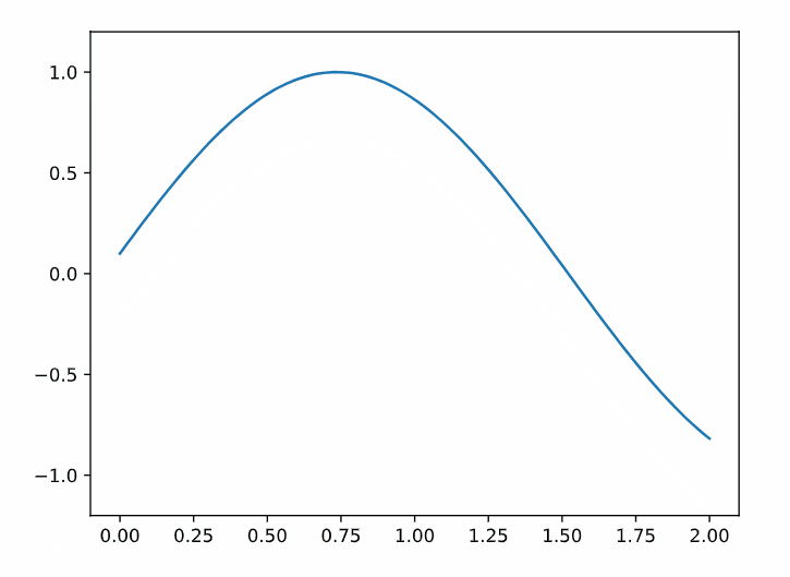
A screenshot of the static Matplotlib figure
In addition, widgets can be used with state management to create interactive plots.
Expanding on the sinusoidal example, freq and phase can be
combined with set_freq, set_phase, and solara.use_state() to
establish these variables as dependencies for
solara.FigureMatplotlib(). The following two lines are placed inside
the Page() component with a starting value specified inside
solara.use_state():
freq, set_freq = solara.use_state(2.0)      # sets the initial value for `frequency`
phase, set_phase = solara.use_state(0.1)    # sets the inital value for `phase`
Next, slider widgets are added for interactive selectability of freq
and phase values for the figure. The on_value argument is paired
with the appropriate set_ variables defined above.
solara.FloatSlider("Frequency", value=freq, on_value=set_freq, min=0, max=10)
solara.FloatSlider("Phase", value=phase, on_value=set_phase, min=0, max=np.pi, step=0.1)
These can now be incorporated into the Page() component and linked
to the figure by including the argument dependencies=[freq, phase]
inside solara.FigureMatplotlib().
In the following code, solara.FigureMatplotlib() is placed inside a
vertical box container. Using return main will return all pieces
inside the main container and does not need to be separately
returned.
import solara
from matplotlib.figure import Figure
import numpy as np

x = np.linspace(0, 2, 100)

@solara.component
def Page():
    # sinusoidal equation and reactive values
    freq, set_freq = solara.use_state(2.0)      # sets the initial value for `frequency`
    phase, set_phase = solara.use_state(0.1)    # sets the inital value for `phase`
    y = np.sin(x * freq + phase)

    # create figure directly
    fig = Figure()              # empty figure
    ax = fig.subplots()         # add axes
    ax.plot(x, y)               # plot equation
    ax.set_ylim(-1.2, 1.2)      # set axes limit

    # vertical box container
    with solara.VBox() as main:
        # generate widgets for interactive selection of dependencies
        solara.FloatSlider("Frequency", value=freq, on_value=set_freq, min=0, max=10)
        solara.FloatSlider("Phase", value=phase, on_value=set_phase, min=0, max=np.pi, step=0.1)
        # generate Matplotlib figure with reactive dependencies
        solara.FigureMatplotlib(fig, dependencies=[freq, phase])
    return main

# the following line is only necessary inside Jupyter notebook to render Page components
display(Page())
A gif of the reactive Matplotlib figure
Altair
Solara supports Altair, a declarative statistical visualization library for Python, and renders figures using VegaLite. See additional details here and here.
The following code outlines the arguments that can be passed through
solara.FigureAltair().
@solara.component
def FigureAltair(
    chart,                                      # altair chart
    on_click: Callable[[Any], None] = None,     # callback function handler for click events
    on_hover: Callable[[Any], None] = None,     # callback function handler for hover events
):

    ...
Inside the Page() component, data will need to be placed into an
Altair chart using chart = alt.Chart() before it can then be
displayed using solara.AltairChart().
chart = alt.Chart(df)
solara.AltairChart(chart)
The following code is a basic example to visualize an Altair chart.
import solara
import altair as alt
import pandas as pd
from vega_datasets import data  # to select sample dataset for this example

# select sample dataset
source = data.seattle_weather()

@solara.component
def Page():
    chart = alt.Chart(source)
    solara.AltairChart(chart)

# the following line is only necessary inside Jupyter notebook to render Page components
display(Page())
bqplot
Solara also supports the bqplot library. Bqplot is a 2D visualization system for Jupyter, based on the constructs of Grammar of Graphics, where each plot component is an interactive widget that can be combined with other Jupyter widgets.
In addition to calling solara and any other dependencies, use
import reacton.bqplot to utilize the bqplot library.
import reacton.bqplot as bqplot # or `as bq` for even further abbreviation
The following example generates a bqplot with widgets for
logarithmic scaling and exponential transformation of a given line.
import solara
import numpy as np
import reacton.bqplot as bqplot

x = np.linspace(0, 2, 100)

# define reactive state variables to initialize
exponent = solara.reactive(1.0)
log_scale = solara.reactive(False)

@solara.component
def Page(ymax=5):           # ymax is defined inside `()` but can also be placed elsewhere
    y = x**exponent.value
    color = "red"
    display_legend = True
    label = "bqplot graph"

    # add interactive widgets
    solara.SliderFloat(value=exponent, min=0.1, max=3, label="Exponent")
    solara.Checkbox(value=log_scale, label="Log scale")

    # customize axes
    x_scale = bqplot.LinearScale()
    if log_scale.value:
        y_scale = bqplot.LogScale(min=0.1, max=ymax)
    else:
        y_scale = bqplot.LinearScale(min=0, max=ymax)

    # create bqplot
    lines = bqplot.Lines(x=x, y=y, scales={"x": x_scale, "y": y_scale}, stroke_width=3, colors=[color], display_legend=display_legend, labels=[label])
    x_axis = bqplot.Axis(scale=x_scale)
    y_axis = bqplot.Axis(scale=y_scale, orientation="vertical")
    bqplot.Figure(axes=[x_axis, y_axis], marks=[lines], scale_x=x_scale, scale_y=y_scale, layout={"min_width": "800px"})

# the following line is only necessary inside Jupyter notebook to render Page components
display(Page())
A gif of a bqplot rendered using Solara
Echarts
Solara can also create ECharts figures. Apache ECharts is an open-source JavaScript visualization library. Solara does not support Python API to create figure data and can only create ECharts figures with provision of data in a specified format. Examples can be found through EChart examples and on Solara’s EChart documentation page.
SQL Integration
Solara offers a SQL-specific textfield input that includes auto-complete and syntax highlighting. See details here.